time_lag
- hydrostats.analyze.time_lag(merged_dataframe: DataFrame, metrics: Sequence[str], interp_freq: str = '6h', interp_type: Literal['linear', 'time', 'index', 'values', 'nearest', 'zero', 'slinear', 'quadratic', 'cubic', 'barycentric', 'polynomial', 'krogh', 'piecewise_polynomial', 'spline', 'pchip', 'akima', 'cubicspline', 'from_derivatives'] = 'pchip', shift_range: tuple[int, int] = (-30, 30), mase_m: int = 1, dmod_j: float = 1, nse_mod_j: float = 1, h6_mhe_k: float = 1, h6_ahe_k: float = 1, h6_rmshe_k: float = 1, d1_p_obs_bar_p: float | None = None, lm_x_obs_bar_p: float | None = None, replace_nan: float | None = None, replace_inf: float | None = None, remove_neg: bool = False, remove_zero: bool = False, plot: bool = False, plot_title: str = 'Metric Values as Different Lags', ylabel: str = 'Metric Value', xlabel: str = 'Number of Lags', save_fig: str | None = None, figsize: tuple[int, int] = (10, 6), station: str | None = None) tuple[DataFrame, DataFrame]
Check metric values between simulated and observed data at different time lags.
Runs a time lag analysis to check for potential timing errors in the simulated data. Can also create a plot using matplotlib of the metric values at different shifts.
- Parameters:
merged_dataframe – A pandas dataframe that has two columns of predicted data (Col 0) and observed data (Col 1) with a datetime index.
metrics – Metric abbreviations that the user would like to use in their lag analysis. Each metric function has a property that contains their abbreviation for convenience (see example).
interp_freq – Frequency of the interpolation for both the simulated and observed time series.
interp_type – Type of interpolation. Options are ‘linear’, ‘pchip’, or ‘cubic’.
shift_range – If given, specifies the range of the lag shifts. For example, if (-10, 10) was given, the function would shift the simulated array for all of the range between -10 and 10.
mase_m – Parameter for the mean absolute scaled error (MASE) metric.
dmod_j – Parameter for the modified index of agreement (dmod) metric.
nse_mod_j – Parameter for the modified Nash-Sutcliffe (nse_mod) metric.
h6_mhe_k – Parameter for the H6 (MHE) metric.
h6_ahe_k – Parameter for the H6 (AHE) metric
h6_rmshe_k – Parameter for the H6 (RMSHE) metric
d1_p_obs_bar_p – Parameter fot the Legate McCabe Index of Agreement (d1_p).
lm_x_obs_bar_p – Parameter for the Lagate McCabe Efficiency Index (lm_index).
replace_nan – If given, indicates which value to replace NaN values with in the two arrays. If None, when a NaN value is found at the i-th position in the observed OR simulated array, the i-th value of the observed and simulated array are removed before the computation.
replace_inf – If given, indicates which value to replace Inf values with in the two arrays. If None, when an inf value is found at the i-th position in the observed OR simulated array, the i-th value of the observed and simulated array are removed before the computation.
remove_neg – If True, when a negative value is found at the i-th position in the observed OR simulated array, the i-th value of the observed AND simulated array are removed before the computation.
remove_zero – If true, when a zero value is found at the i-th position in the observed OR simulated array, the i-th value of the observed AND simulated array are removed before the computation.
plot – If True, a plot will be created that visualizes the different error metrics at the different time lags.
plot_title – If the plot parameter is true, this parameter will set the title of the plot.
ylabel – If the plot parameter is true, this parameter will set the y axis label of the plot.
xlabel – if the plot parameter is true, this parameter will set the x axis label of the plot.
save_fig – If given, will save the matplotlib plot to the specified directory with the specified file name (e.g. /path/to/plot.png). A list of all available types of figures is given in List of Plot File Types.
figsize – Tuple that specifies the horizontal and vertical lengths of the plot, in inches.
station – The station of analysis. Includes the station in the table if given.
Notes
If desired, users can export the tables to a CSV or Excel Workbook. This can be done using the built in methods of pandas. A link to CSV method can be found at https://pandas.pydata.org/pandas-docs/stable/generated/pandas.DataFrame.to_csv.html, and a link to the Excel method can be found at https://pandas.pydata.org/pandas-docs/stable/generated/pandas.DataFrame.to_excel.html
- Returns:
The first DataFrame contains all of the metric values at different time lags, while the
second dataframe contains the maximum and minimum metric values throughout the time lag,
and the index of the maximum and minimum time lag values.
Examples
Using data from the Streamflow prediction tool RAPID model and the ECMWF model, we can compare the two at different time lags
>>> import hydrostats.analyze as ha
>>> import hydrostats.data as hd
>>> from hydrostats.metrics import me, r_squared, rmse, kge_2012, nse, dr
>>>
>>> # Defining the URLs of the datasets
>>> sfpt_url = r"https://github.com/waderoberts123/Hydrostats/raw/master/Sample_data/sfpt_data/magdalena-calamar_interim_data.csv"
>>> glofas_url = r"https://github.com/waderoberts123/Hydrostats/raw/master/Sample_data/GLOFAS_Data/magdalena-calamar_ECMWF_data.csv"
>>> # Merging the data
>>> merged_df = hd.merge_data(sfpt_url, glofas_url, column_names=("SFPT", "GLOFAS"))
There are two dataframes that are returned as part of the analysis.
>>> # Running the lag analysis, not that HydroErr > 1.24 must be used to access the .abbr
... # property
>>> time_lag_df, summary_df = ha.time_lag(
...     merged_df,
...     metrics=[me.abbr, r_squared.abbr, rmse.abbr, kge_2012.abbr, nse.abbr],
... )
>>> summary_df
                    Max  Max Lag Number          Min  Min Lag Number
ME           174.740510           -28.0   174.740510           -24.0
r2             0.891854            -2.0     0.646193           -30.0
RMSE        3142.795474           -30.0  1754.455598            -2.0
KGE (2012)     0.877116            -2.0     0.775328           -30.0
NSE            0.856358            -2.0     0.539076           -30.0
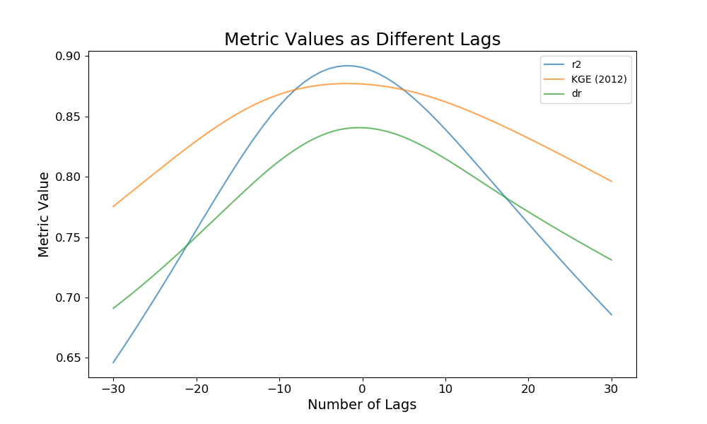
A plot can be created that visualizes the different metrics throughout the time lags. It can be saved using the savefig parameter as well if desired.
>>> _, _ = ha.time_lag(merged_df, metrics=[r_squared.abbr, kge_2012.abbr, dr.abbr], plot=True)